Smart Floor Project
The following is an overview of the SmartCare Project's Smart Floor technology.
Full in-depth details can be found in my dissertation: Learning Health Information From Floor Sensor Data Within A Pervasive Smart Home Environment.
For more information on the SmartCare Project in large, please visit the SmartCare Project Page.
Overview
The goal and purpose of the smart floor is to extract individual foot contact points generated by normal walking behavior. These contact points can be used for Gait Analysis, person identification, tracking, pattern recognition, and anomaly detection.
The current progress consists of four main steps:
- An automatic calibration technique for grouped smart floor sensors that does not require rigid and specific physical effort.
- A multi-stage neural network model that extracts single contact points from a person’s calibrated walking data in a low-resolution environment.
- A recursive Hierarchical Clustering Analysis algorithm to cluster and segment a person's individual footfalls using the model's single contact point output data.
- Using k-nearest neighbors classification to identify people based on Gait Parameters using walking data passed through the previous steps.
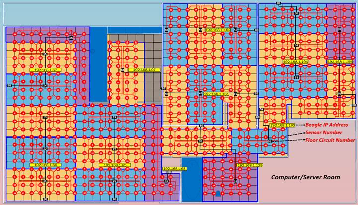
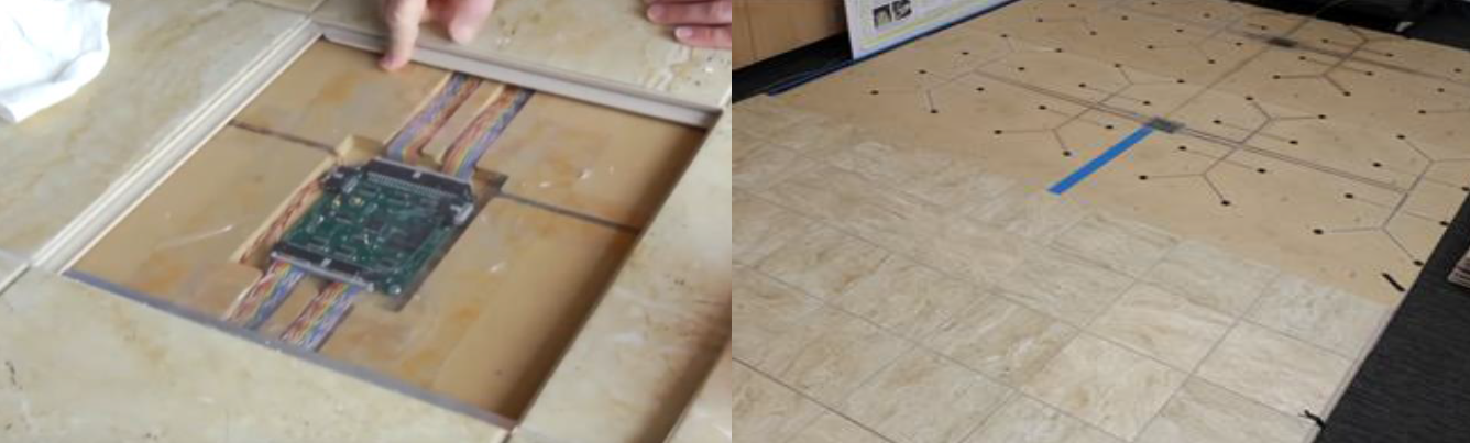
The SmartCare apartment's entire floor is equipped with our custom-built sensor-infused subfloor sitting beneath ceramic tile. A single pressure/force sensor is located at every corner of the 1sqft tile configuration resulting in a resolution of 1 sensor per 1 square foot. There are a total of 712 floor sensors covering the entire apartment.
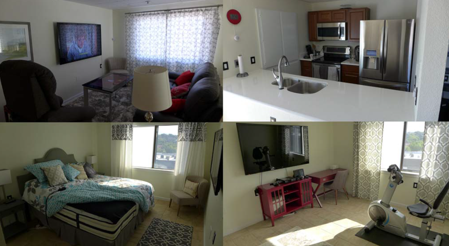
The uniqueness of the SmartCare project, in terms of the floor, is its size, coverage, rigid tile surface, and low-cost. Other floor sensor projects either use off-the-shelf high-resolution mats or small custom-built smart floors that only exist in labs. Deploying enough high-resolution mats to cover the entire area of the SmartCare apartment is cost prohibitive. While the SmartCare floor requires specialized knowledge and labor to create and install, the price tag is magnitudes cheaper than purchasing enough high-resolution mats to cover an equal amount of space. Also, the large sensor-array floor is deployed within an actual living environment, not just a lab solely used for experiments. The smart floor captures real-time data of individuals living their normal lives within a typical apartment. This helps eliminate or reduce the white coat hypertension effect someone may experience if asked to walk on a floor subsection within a lab or health facility while being analyzed.
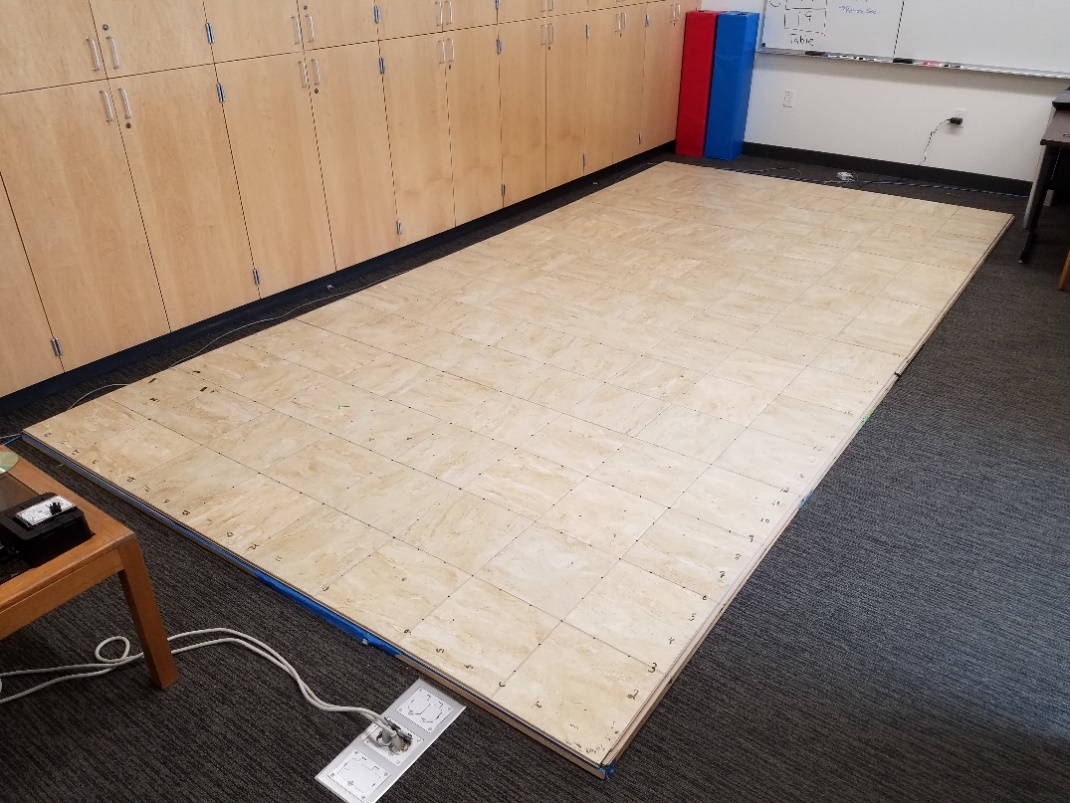
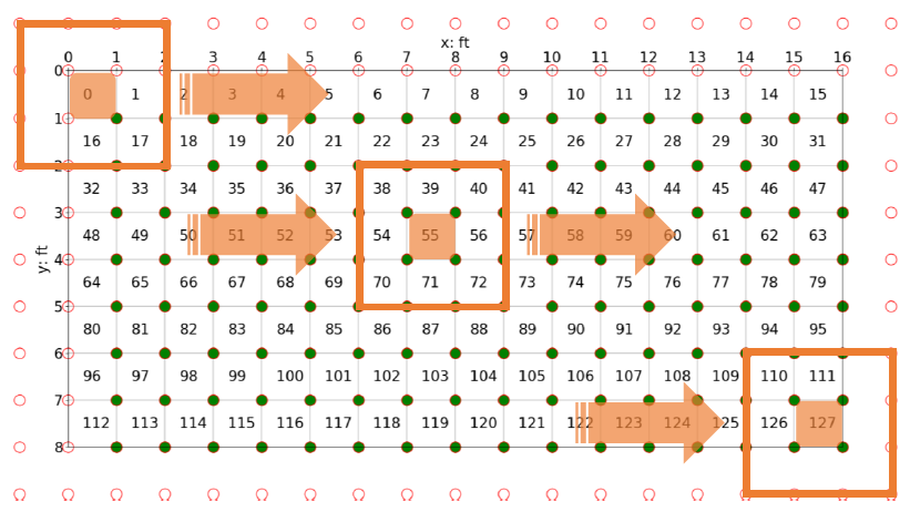
A smaller smart floor was built on campus at UTA for experimentation and software development. The 16ft x 8ft lab floor consists of only 128 pressure sensors.
Automatic Floor Sensor Calibration
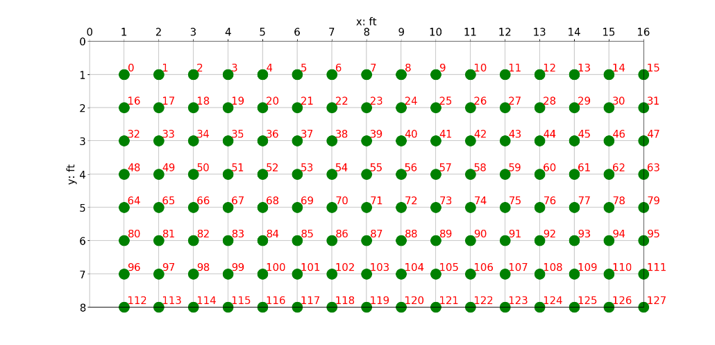
Using a top-left origin approach, the sensor indexing i for the 128 sensors of the lab floor begins at the top left corner and ends at the bottom right corner. The floor sensor’s data is collected at 25Hz, therefore each time index t represents 1/25 of a second. The embedded circuity and microcontroller samples each pressure sensor, performs a 10-bit analog-to-digital conversion (ADC), and returns a whole number integer value ranging from 0 to 1023. This raw sensor value s is what must be calibrated and translated to known weight units (kg). Through experimentation the pressure sensor exhibited linear behavior when increasing, known weights were applied, and outputted a value of 0 when no weight was applied (0 kg).
The following notation for key terms is used for the calibration process of the lab's smart floor:
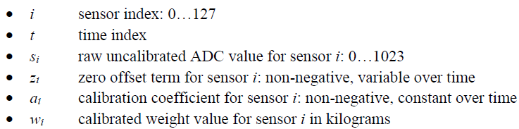
While a traditional calibration approach of using the simple linear equation y = mx + b to translate raw sensor values in kgs is feasible for calibrating standalone sensors independently, it is too limited for an interconnected sensor grid underneath a shifting tile floor. The weight to be captured on top of the floor spreads across multiple tiles and sensors. Also, the tile coupling, shifting, and flexing over time in the x, y, or z directions can shift the constant tile weight offset b each sensor experiences. Constant recalibration would have to be applied to find the new updated a and b values to account for any day-to-day tile floor changes.
A more practical approach for this floor system would be to automatically remove the constant non-human unloaded weight seen by the sensor so only a single term a is required to be calculated. The term unloaded weight describes sources of weight we are not interested in knowing or capturing. This ever-changing weight could be tile, furniture, or temporary non-human objects. For example, if a 90 kg person’s whole home is fitted with this floor tile sensor system, standing freely in the kitchen should yield the same weight calculation result as when they are sitting on a couch in the living room. The constant weight of the couch should be filtered out so only the person’s weight is captured and converted to kg. To achieve this, a z offset term needs to be subtracted from the ADC sensor value s over time. This z value fluctuates to account for constant weight being added or removed on or near the sensor in question. Once the sensor’s s value has had its z offset removed, linear regression in the form of OLS can be applied to learn each sensor’s a value.
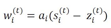
The calibrated weight w experienced by the single sensor i at time t is expressed as:
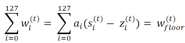
Since no sensor is truly independent once it has been placed underneath the tile floor, the calibrated weight experienced by the entire lab floor at time t is expressed as:
Each sensor's state at any time t can be categorized as one of the following:
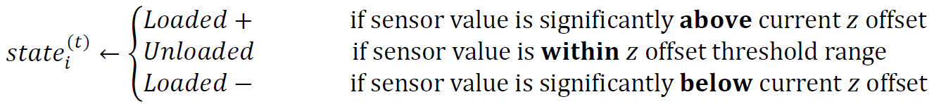
The Unloaded state can be interpreted as no person is contributing to the weight observed by the sensor, only static, non-human objects affect the sensor’s value. Loaded+ signifies a human weight has caused an increase in the sensor value s and should not be filtered out or lumped together with the z offset. Loaded- is a momentary state where the tile’s coupling and the elasticity of the rubber surrounding the sensors causes the sensor to read a lower value than the current z offset level. These are seen as brief negative weights due to the impact forces of a person walking on the tile-covered smart floor. This state’s importance is to more accurately calculate the a scalar during the linear regression process for each sensor during calibration and prevent under or over shooting of the final weight value w.
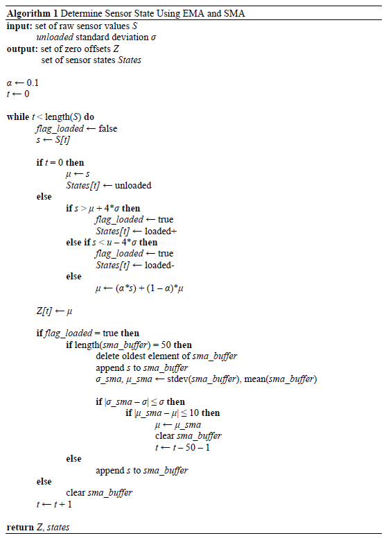
The smart floor sensor calibration process consists of three main steps:
- Find each sensor’s unloaded standard deviation σi used for removing zero offsets and determining sensor states during training and testing
- Find each sensor’s weight coefficient ai that performs the linear transformation from undefined raw sensor values si to kg weight units
- Use σi and ai with new incoming floor data to calibrate and translate sensor values into wi units
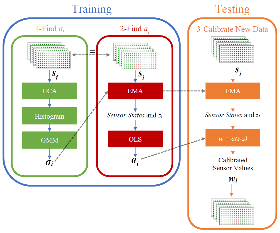
The in-depth details regarding calibration (gaussian mixture models, clustering, exponential moving average, etc.) are found in my dissertation document at the top of this page.
Contact Point Extraction using Machine Learning Techniques
Now the really interesting stuff begins...
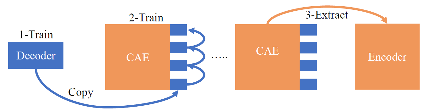
Due to the low 1-sqft resolution of the smart floor, single contact point extraction of a person’s footfalls cannot be achieved as straightforwardly as when using a sensor-dense high-resolution floor or mat. To achieve this extraction while considering the non-linear coupling properties of the floor, a Convolutional Autoencoder Neural Network model is used. The model’s sequential design consists of 3 main steps:
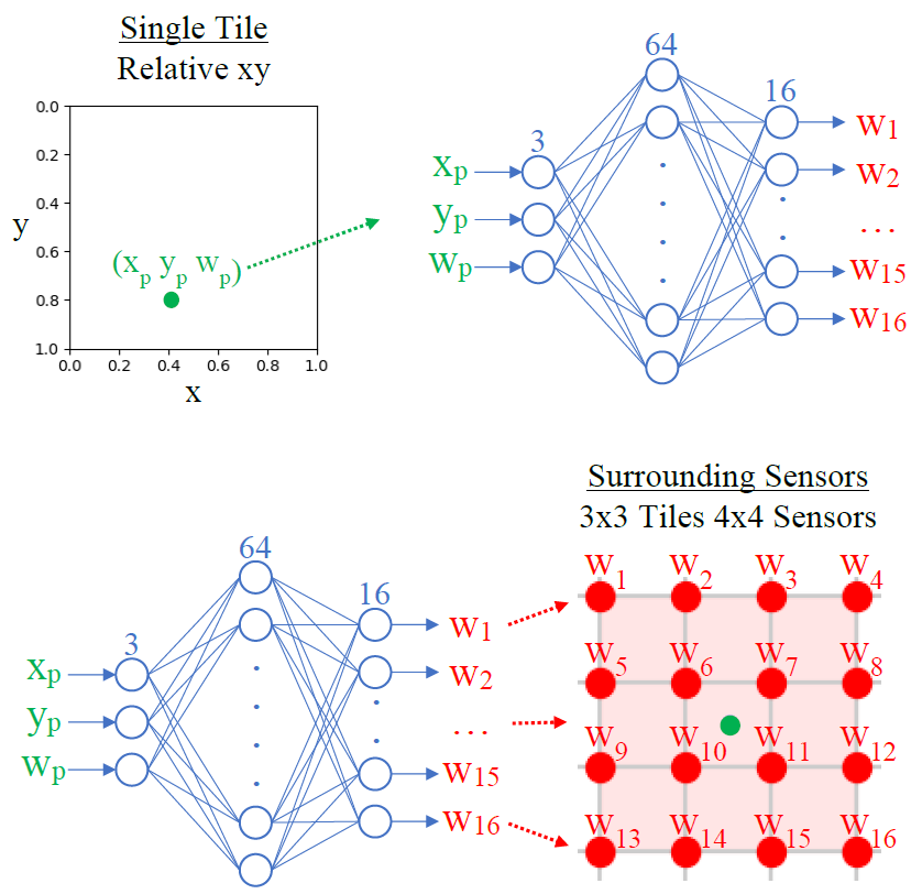
- Design and train the Decoder model which maps known location data and weight to a 4x4 square grid of calibrated sensor values in a supervised fashion. This can be thought of as the Tile Model and is trained with a very specific training dataset.
- Design and train the Convolutional Autoencoder (CAE) model that incorporates 128 copies of the pre-trained Decoder (transfer learning). The convolutional parts of the model learn the non-linear relationships and interactions between sensors, tiles, and how weight spreads on the smart floor. The CAE is trained in a semi-supervised fashion and can be trained with a large amount of arbitrary calibrated walking data.
- After the CAE is fully trained the frontend Encoder portion is extracted and becomes the resulting final model used to translate regular calibrated walking data into a series of individual contact points no longer limited by the low resolution of the smart floor.
The rationale behind this approach to separately train the Decoder and Encoder components addresses the requirement that we want to obtain contact location and weight data and thus the hidden representation of the autoencoder architecture has to be of a specific type which can only be achieved using some level of supervised data. As opposed to supervised training of the Encoder which performs the ultimate contact point extraction task, however, the only supervised training performed here is of the Decoder, which requires significantly less and easier to obtain data. This stems from the observation that sensor pressure values from multiple weights on the floor combine purely additively and thus the sensor reading from multiple weights (contact points) on the floor can be computed by adding the values for each sensor for the Decoders sharing this sensor within their sensor region. This implies that it is possible to train the Decoder using only single contact point calibrated data which is significantly simpler to obtain than multi-contact data.
The Encoder, on the other hand, has the task to split sensor readings into sets of contact points, and thus requires multi-contact data. In the approach used here, the pre-training of the Decoder with single contact point data makes it possible to train the Encoder using unlabeled walking data which does not contain weight and contact point information and is thus significantly simpler to obtain. In addition, this procedure enables one to train the Decoder on a smaller part of the floor while training the encoder to capture the entire floor.
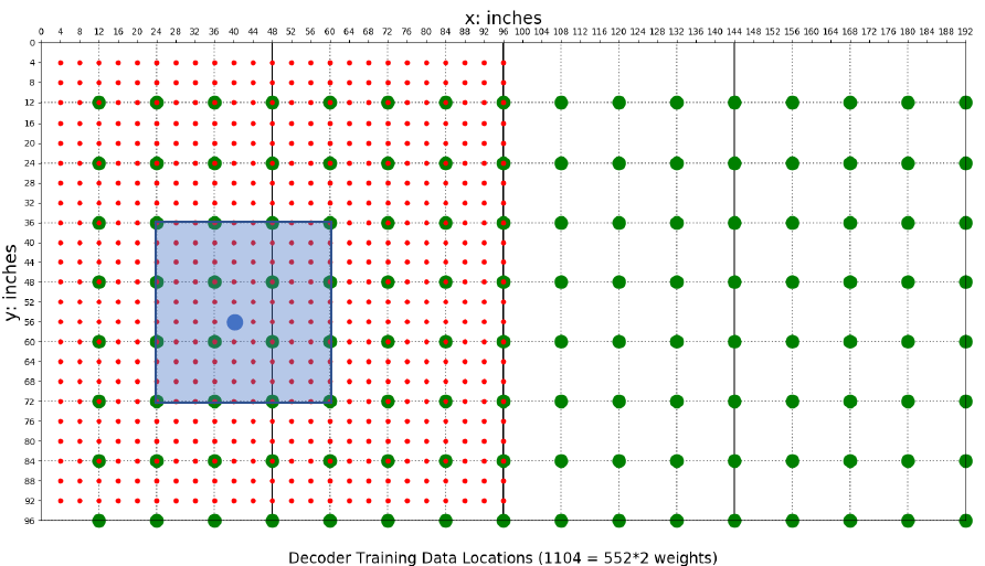
The Decoder is trained from specific training data (indicated by red dots below) where known human weights were recorded. The Decoder is trained in 4x4 sensor chunks (3x3 tiles). The sensor readings feeding the Decoder during training are calibrated using the process described previously.
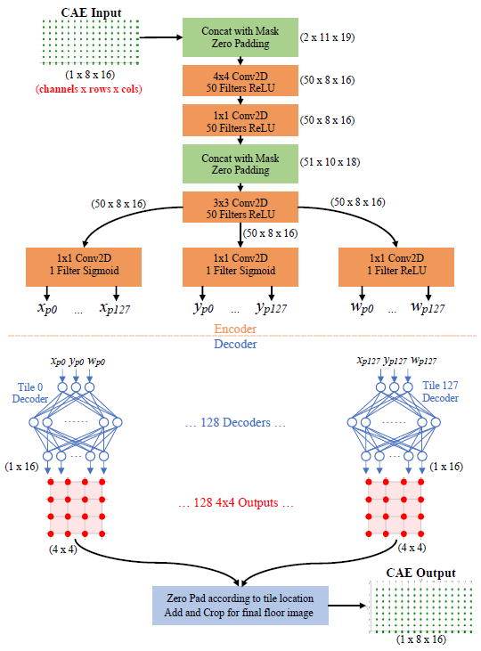
Once the Decoder is trained, it can be integrated into a Convolutional Autoencoder architecture (CAE) while effectively serving as a distal teacher for the encoder portion. The CAE consists of two main parts: the convolutional Encoder portion and the 128 pretrained Decoders, one for each tile. The overlapping Decoders’ outputs for each sensor are added, effectively having the Decoders form a deconvolution transforming multiple contact points to corresponding sensor readings. The weight and bias parameters for the 128 identical Decoder models are frozen and untrainable during the CAE training process. The CAE’s input data and output target data are entire floor snapshots of calibrated sensor data of various walking data from different people. Since the CAE’s main goal is to reconstruct the input data as perfectly as possible, the bottleneck between the two portions forces the CAE, during training, to learn an encoding that adopts the contact point properties embedded within the Decoder.
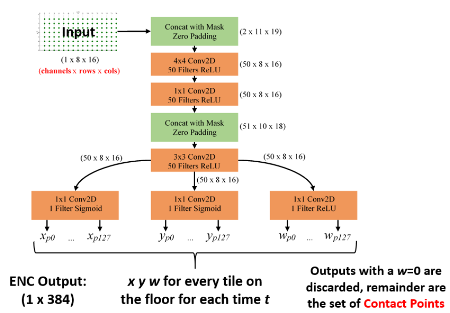
The CAE slides or convolves 4x4 sensor (3x3 tile) kernels over the entire floor and learns how neighboring sections of the floor interact, couple, and affect one another while also trying to recreate the same input pressure profile of the entire floor on its output in adherence to the contact point profile learned in the Decoder’s training process. The stacking with other convolutional layers with differing kernel sizes allows the CAE to see larger segments of the floor and discover more complex non-linear relationships within the smart floor. In other words, the CAE takes a single entire floor snapshot and the Encoder portion outputs an (xp yp wp) for every tile with the wp serving as a probability of sorts. The complete CAE architecture used here uses 3 convolutional layers and additional padding masks to account for the sensor-less edges of the floor. The CAE's training data is simply various walking files of people with different weights (after calibration). The CAE can be trained (for the most part) with unlabeled data while learning the intricate differences and details of how the floor behaves and spreads weight.
However, this straightforward CAE approach proved insufficient and output training targets needed to be reinforced with multiple outputs and activity regularization during the training process. The resulting model is named the SIMO CAE (Single Input Multiple Output Convolutional Autoencoder).
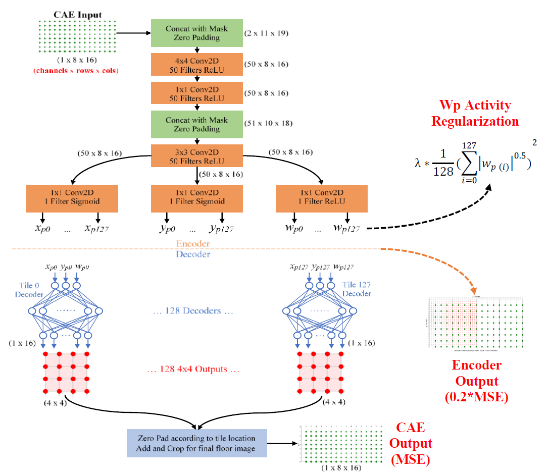
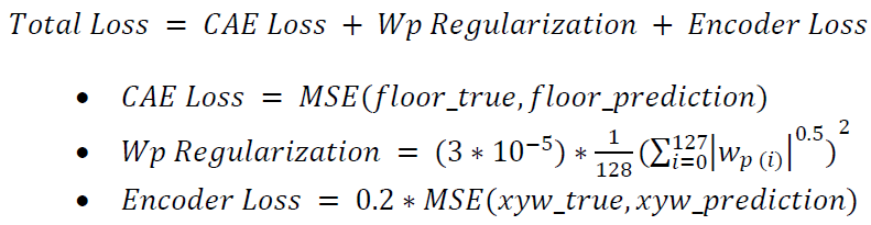
To prevent zero-weight biasing, the CAE Loss single sensor contribution is reduced to 0.01% within the mean squared error function if both true and prediction weight targets are within +/- 1kg of zero weight. The CAE Loss indicates how well the model can reconstruct the entire floor weight. The Wp Regularization acts as a penalty to encourage more single contact point explanations. The Encoder Loss signifies how well the model’s bottleneck can generate accurate contact points per tile. Finally, the Total Loss describes how well the overall model is learning.
After the SIMO CAE is fully trained, the Encoder portion is kept as the final standalone model in predicting individual contact points per tile and across the entire floor. When a series of entire floor snapshots are given to the input of the Encoder, each output is of the shape (1 x 384) which holds the (xp yp wp) values for each of the 128 tiles on the floor. If a tile’s wp value is close to 0kg then that tile’s (xp yp wp) is discarded and only tiles with weight activity are kept. Each final contact point is prepended with timestamp information given from the original series of input data resulting in (t xp yp wp) to describe each contact point.
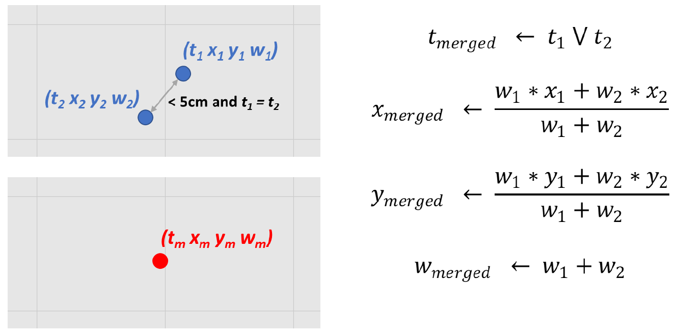
Once only relevant tile contact points remain, they must be converted from relative coordinates to absolute floor coordinate units according to their tile’s location while retaining their original timestamps t and weight values wp, (t xp yp wp) → (t xa ya wa). If there exist multiple contact points at the same time t and if their Euclidean distance is less than 5cm then it is assumed the Encoder incorrectly split contact points at tile boundaries and they should be recombined. The new combined xa ya location is chosen based off each points wp weight value instead of merely splitting the difference.
Footfall Clustering and Gait Analysis
After the absolute contact points are successfully extracted using the Encoder model, they are clustered to segment individual footfalls of a person while also removing outliers. A time series of k contact points is expressed as:

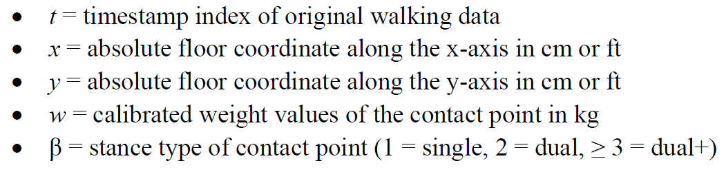
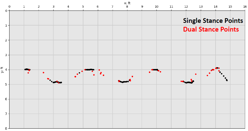
The 25Hz sample rate of the floor is fast enough to capture the moment two feet are in contact with the floor at the same time even at a brisk walk. Stance type β is a variable to help describe which support phase (single or double) a contact point belongs to when a person is walking. Labeling contact points as dual stance type can also support segmenting and signifying the start or end of an individual footfall. Contact point data of dual+ stance type was deemed Encoder output outliers and were discarded before foot clustering began. Stance type was determined by counting the number of shared contact points at timestamp t within the CP data.
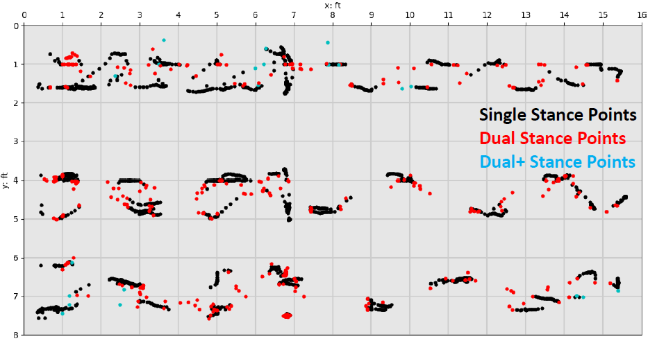
The first figure below shows an entire walking sequence of multiple passes over the entire floor with single stance points in black, dual in red, and dual+ in cyan while the 2nd figure shows the same for a single walking pass.
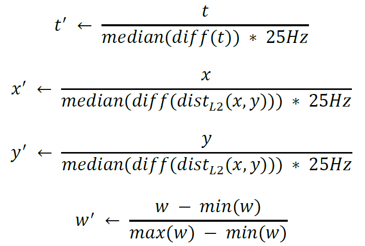
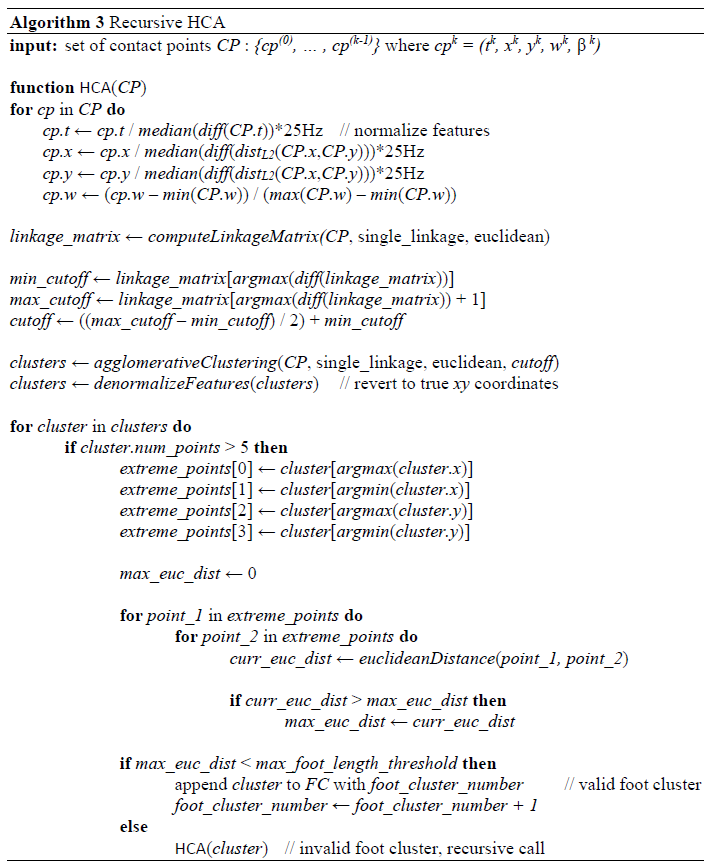
Before Hierarchical Clustering Analysis (HCA) is performed to determine the clusters representing individual footfalls, contact point features are normalized. The stance type β is not used for HCA and therefore not normalized here. The CP features t, x, and y are scaled according to each feature’s median rate of change considering the time between two consecutive floor samples taken at 25Hz (1/25Hz = 0.04sec). Additionally, location features x and y are jointly normalized using the Euclidean distance of their sequential differences to avoid axis bias in case one direction was spanned differently than the other during an entire walking sequence. Weight feature w is normalized with the standard min-max method [0…1]. Below, diff() represents finding the sequential n-th order discrete difference along the feature column.
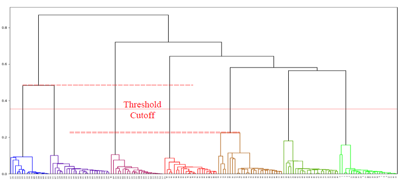
Recursive Hierarchical Clustering Analysis
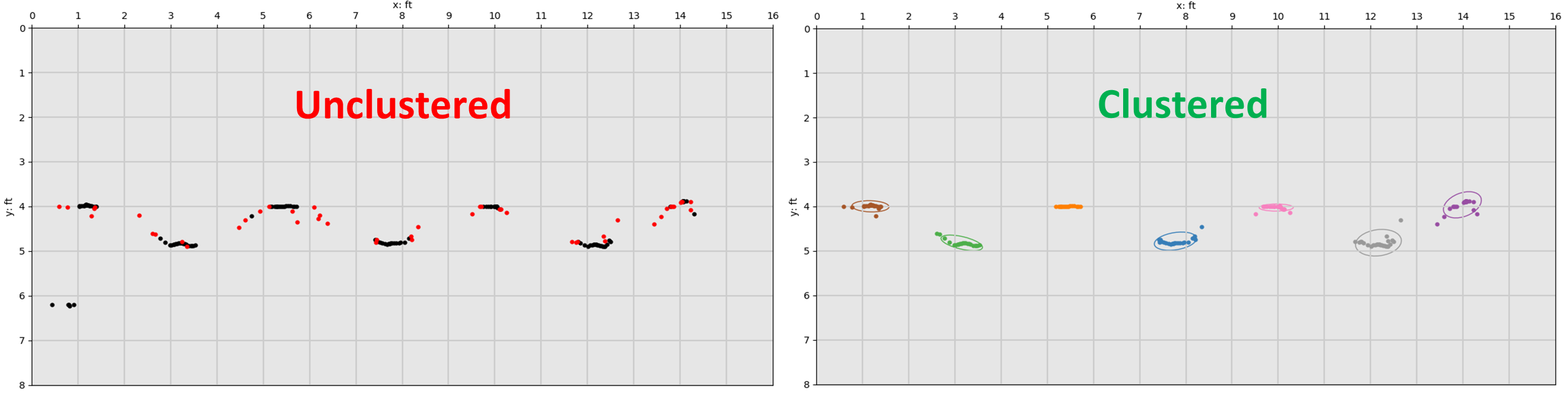
Using the normalized feature vectors of all contact points, HCA (agglomerative method) is performed to segment and cluster points together into individual foot falls using minimum linkage and Euclidean distance for the distance metric. When viewing the results of an HCA as a dendrogram, the middle of the largest vertical distance between a cluster merge is picked as the criterion to “best cut” the tree and decide how many clusters is optimal. In practice this is achieved by finding the largest jump in the computed linkage matrix. Since a single global “best cut” spanning the entire dendrogram does not guarantee finding each individual footfall cluster, local “best cuts” must be found within groupings of groupings deep within the tree. The recursive element of the HCA foot clustering algorithm will continue to further split clusters with the same “best cut” method until the max Euclidean distance within a cluster is under a maximum “foot length” threshold of 35.56 cm (14 in) while also discarding clusters that contain fewer than 5 individual contact points (single observations).
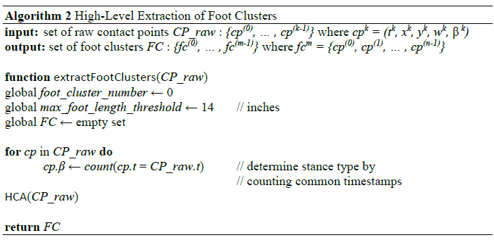
After a set of m foot clusters are found (FC = {fc(0), fc(1), … , fc(m-1)} where fcm = {cp(0), cp(1), … , cp(n-1)} and cpn = (tn, xn, yn, wn, βn)), if there exists any dual stance points who’s pair is within the same cluster they are merged together and become single stance type. If a dual stance point’s pair belongs to another foot cluster they are left unchanged. Algorithm 2 shows a high-level view of the foot-cluster extraction process and Algorithm 3 shows in more detail the recursive hierarchical clustering approach.
Segmenting into Gait Sequences
Once foot clusters are found, gait sequences can be constructed for follow-up gait parameter extraction. For this, all foot clusters are sorted according to the mean t of each cluster’s set of contact points. The entire set of foot clusters FC must be segmented into a set of gait sequences where reliable gait parameters can be extracted. This involves separating gait sequences if a person physically leaves the floor and returns and when a walking person is making a turn. Extracting step, stride, and other gait parameters during a turning sequence is deemed unreliable and only gait sequences where a person walks semi-straight are to be used.
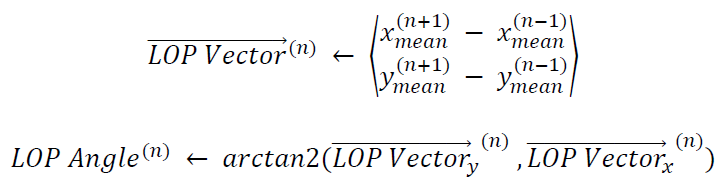
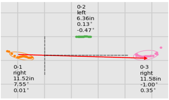
If there exists a time gap of at least 1.5 secs in the sequential set of foot clusters, it is assumed the person has left the smart floor and the foot clusters are separated into different gait sequences. Within each gait sequence, a local line of progression (LOP) is calculated for each stride using sets of 3 sequential footfalls fc(n-1), fc(n), and fc(n+1). The LOP vector is drawn between the xy mean of the 1st and 3rd foot clusters as they should represent the same foot. The LOP angle for the middle foot cluster fc(n) is calculated by applying the arctan2() function on the LOP vector. The LOP angles for the first and last foot cluster within a gait sequence are merely the copy of the closest neighbor since those feet do not exist within the “middle” of a complete stride. The figure below shows the LOP and foot angles for a sequence of 3 foot clusters.
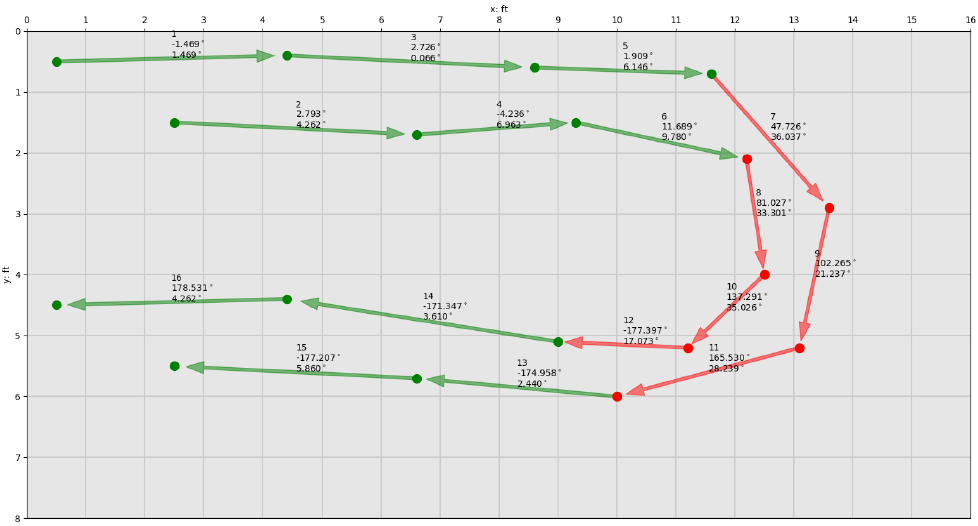
The LOP angles of each foot cluster are used to determine whether a person is walking semi-straight or turning on the smart floor. Iterating sequentially over the set of foot clusters in pairs, if the absolute difference between each foot cluster’s LOP angle is greater than 10 degrees, then the latter of the two is labeled a turn. This comparison is performed for all foot clusters and the gait sequence is further split into more gait sequences wherever turns are found. The turn data is not thrown out since it offers location data that could be useful for tracking, but they are not used in the subsequent gait analysis. The figure below shows sample data of an initial lone gait sequence split into two after turns were discovered within the walking path, indicated in red. During this time and turn splitting process, if a resulting gait sequence contains less than 3 total foot clusters then it is discarded since meaningful gait parameters require many sequential footfalls to calculate.
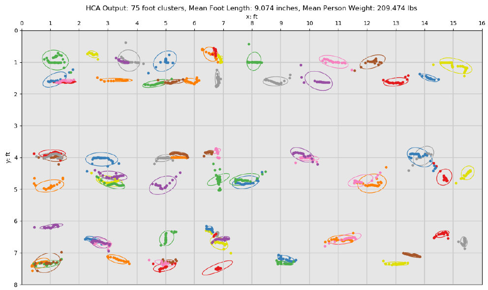
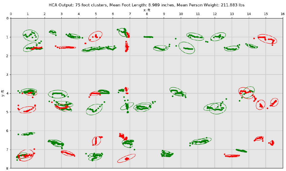
The 1st figure below shows an example of the foot clusters of a person walking across the floor in multiple passes with turns before gait sequence extraction and identification of turns. Based on these clusters, the 2nd figure shows the classification of foot clusters into straight and turn types, clearly identifying the straight line passes and the separating turns between them.
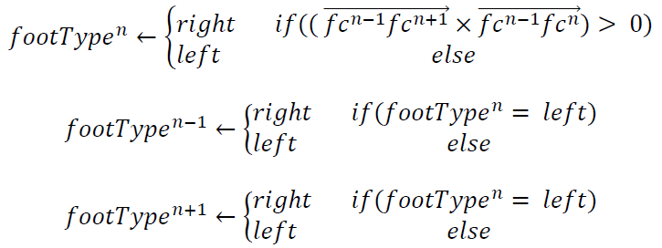
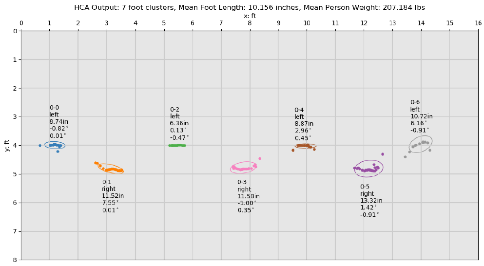
After each gait sequence’s foot clusters are finalized, each foot cluster is labeled as right or left. This process assumes the person is walking forward. Using sets of 3 sequential foot clusters fc(n-1), fc(n), and fc(n+1) the middle foot cluster’s left/right foot type is determined by using the sign of the cross product of the vectors from fc(n-1) to fc(n+1) and fc(n-1) to fc(n). The vectors span to the xy mean of each foot cluster. Using known data and intuition, a positive sign indicated the middle fc(n) is a right foot and negative indicated left. The small algorithm also labels fc(n-1) to fc(n+1) the opposite of the found fc(n) label. This process iterates over the entire gait sequence until all foot clusters are labeled with a foot type, resulting in the identification illustrated in the figure below.
Gait Analysis
After each gait sequence only contains semi-straight walking segments without turns and each foot cluster’s footType and LOP angle are calculated, gait analysis can be performed. Each gait sequence will generate 20 total gait parameters (10 left, 10 right): foot weight, foot length, foot angle, step length, stride length, step width, step time, step speed, stride time, and stride speed.
Foot Weight
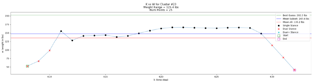
Each foot cluster’s weight (kg) is calculated by finding the mean of the middle 50% of the sorted single contact point calibrated weight values in kg. Only computing the mean weight on the middle subset helps to exclude any valid dual stance points who usually exhibit a smaller weight since they are paired with another contact point also in contact with the floor at the same time. This also helps to remove heel strike and toe off moments where weight spikes might occur due to downward forces while walking.
Foot Length
A cluster’s foot length (cm) is calculated by finding the maximum Euclidean distance between the set of the most extreme xy points within the cluster.
Foot Angle
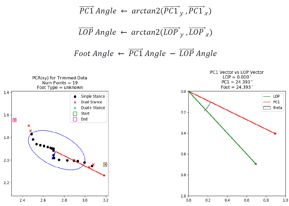
A cluster’s foot angle (degrees) is calculated using the LOP vector of the cluster and the principal component of the contact points within the foot cluster. Principal Component Analysis (PCA) is performed on the set of xy contact points minus any dual stance points detected at the start or end of the foot cluster. These points are not included so the predominant contributing factor to the principal component, and ultimately the foot angle, is the stable region during the mid-stance portion of the gait cycle when the foot is most flat with the floor and gives the most accurate description of direction and angle. After PCA is performed on the xy data, the unit vector of the principal component PC1 is compared against the LOP vector to calculate the foot cluster’s angle.
Step Length
Two sequential foot clusters are required to calculate a step length (cm), fc(n) and fc(n+1). The toe-off xy points of both clusters and the LOP vector from the second cluster are needed. The toe-off points are determined to be the last xy coordinate in the time-sorted set of contact points per foot cluster. Step length is not measured by absolute xy Euclidean distance of the two toe-off points, it is measured along the line of progression (LOP) the person is walking. The toe-off points of both clusters are projected on to the LOP line found using the LOP vector’s slope and y-intercept. The LOP vector is found using cluster xy means, not toe-offs so both have to be projected. The final step length is the Euclidean distance between the projected toe-off points of both clusters. The step length’s left/right label matches the footType label of the fc(n+1) cluster, the foot that travelled the distance to complete the step.
Stride Length
Two toe-off points of sequential foot clusters of the same type, left or right, are required to calculate the stride length (cm), fc(n) and fc(n+2). The LOP vector of the middle cluster fc(n+1) is used for projecting the toe-off points. With these values the stride length calculation follows the same procedure as step length.
Step Width
Step widths (cm) are calculated by iterating over every foot cluster one-by-one excluding the first and last. Each foot cluster’s xy mean point is projected onto its own LOP vector and the projected point’s travel distance is the step width. The step width’s left/right label matches that of the foot cluster in question.
Step Time
Step time (seconds) is calculated by using the same foot clusters for calculating step length. The step time is merely the difference in timestamp t values between the two toe-off contact points divided by the smart floor’s data sampling rate of 25Hz.
Step Speed
Step speed (cm per sec) is calculated by iterating over each step length and dividing by its respective step time pair.
Stride Time
Stride time (seconds) is calculated by using the same foot clusters for calculating stride length. The stride time is merely the difference in timestamp t values between the two toe-off contact points divided by the smart floor’s data sampling rate of 25Hz.
Stride Speed
Stride speed (cm per sec) is calculated by iterating over each stride length and dividing by its respective stride time pair.
Gait Parameter Means and Variances
If the walking sequence is sufficiently large means and variances over the entire dataset of gait values are calculated. For each of the 20 gait features, the middle 50% of the sorted feature vector is used to calculate the mean and variance to help remove any small or large outliers. The figures below show examples of the calculated gait features for a single pass and a set of passes, respectively.
Preliminary Person Identification
Another experiment was performed to evaluate the utility of the extracted gait parameters and their ability to distinguish different gait patterns. In particular, a person identification classifier was trained using only the extracted gait parameters from the smart floor data. For this, k-nearest neighbors (k-NN) classification was applied to the smart floor’s gait parameter calculations from the subjects’ data in the walking study. This preliminary effort of person identification based solely off gait parameters used standard k-NN techniques without special weighting schemes.
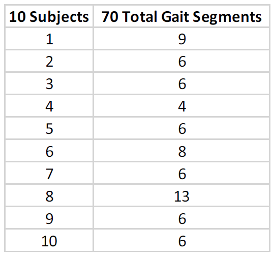
Each of the 10 unique individuals generated 4 to 13 valid gait segments during their full walking sequence across the entire floor. A total of 70 valid gait segments across all subjects were generated. A valid gait segment contains at least four footfalls after gait segmentation due to turns and leaving the floor. The minimum requirement of four footfalls ensures that every gait parameter has enough data for a calculation (i.e. left and right strides). The feature space for each sample is the 20 gait parameter means from each valid gait segment.
Note that previously established subject 0 is the same person as subject 8, and the two datasets have been combined and labeled solely as 8. The k-NN class labels are the 10 subject numbers (IDs).
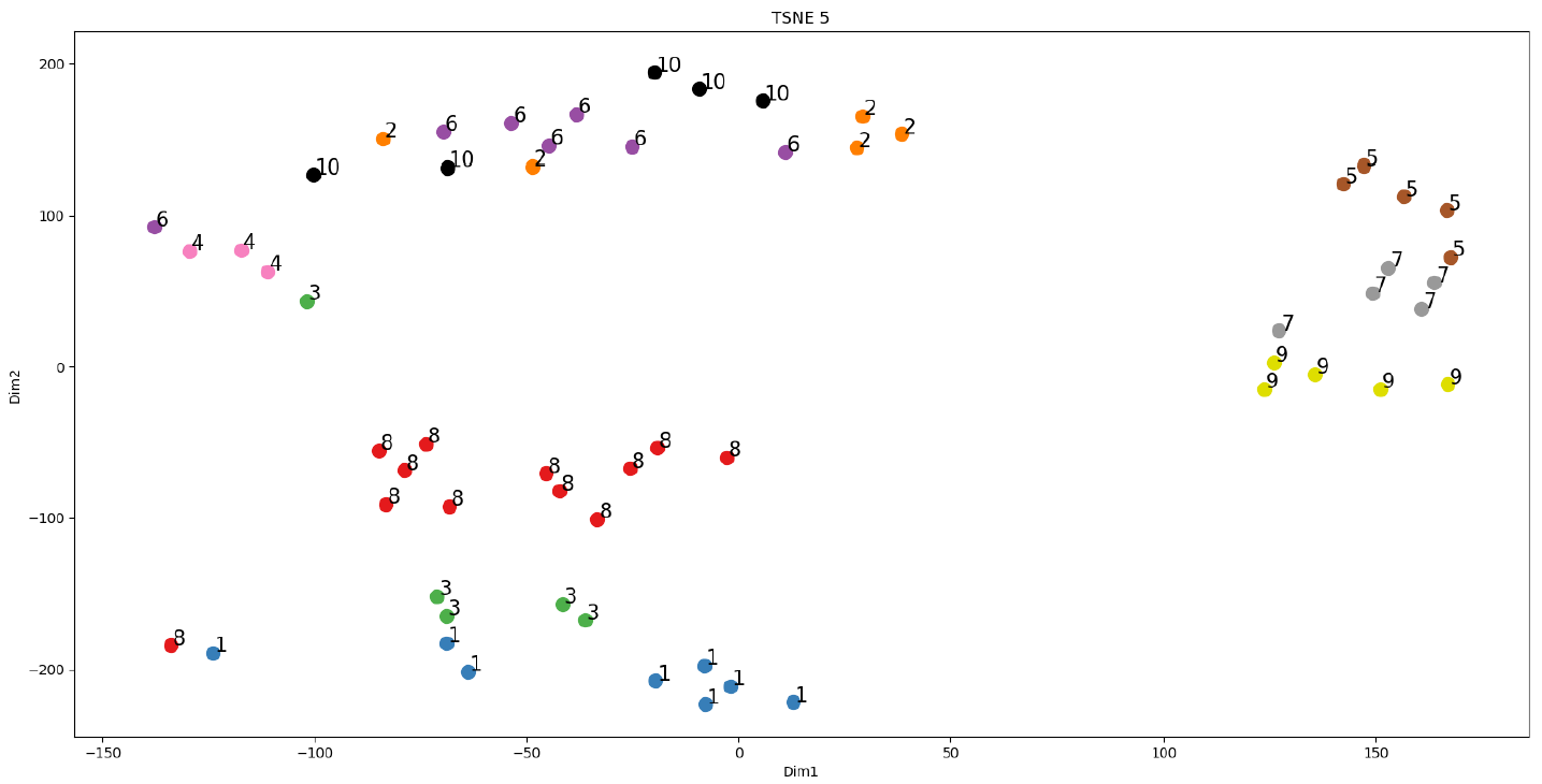
The figure below shows the 20-dimensional feature space of each gait segment sample reduced to 2 dimensions using t-distributed stochastic neighbor embedding (t-SNE). It is purely for visualizing the high-dimensional data and is not used in the k-NN algorithm. A perplexity of 5 was used for the t-SNE plot.
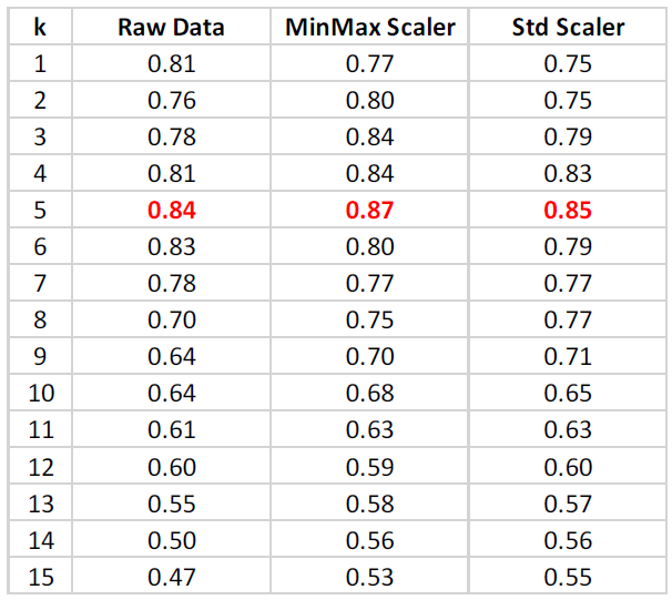
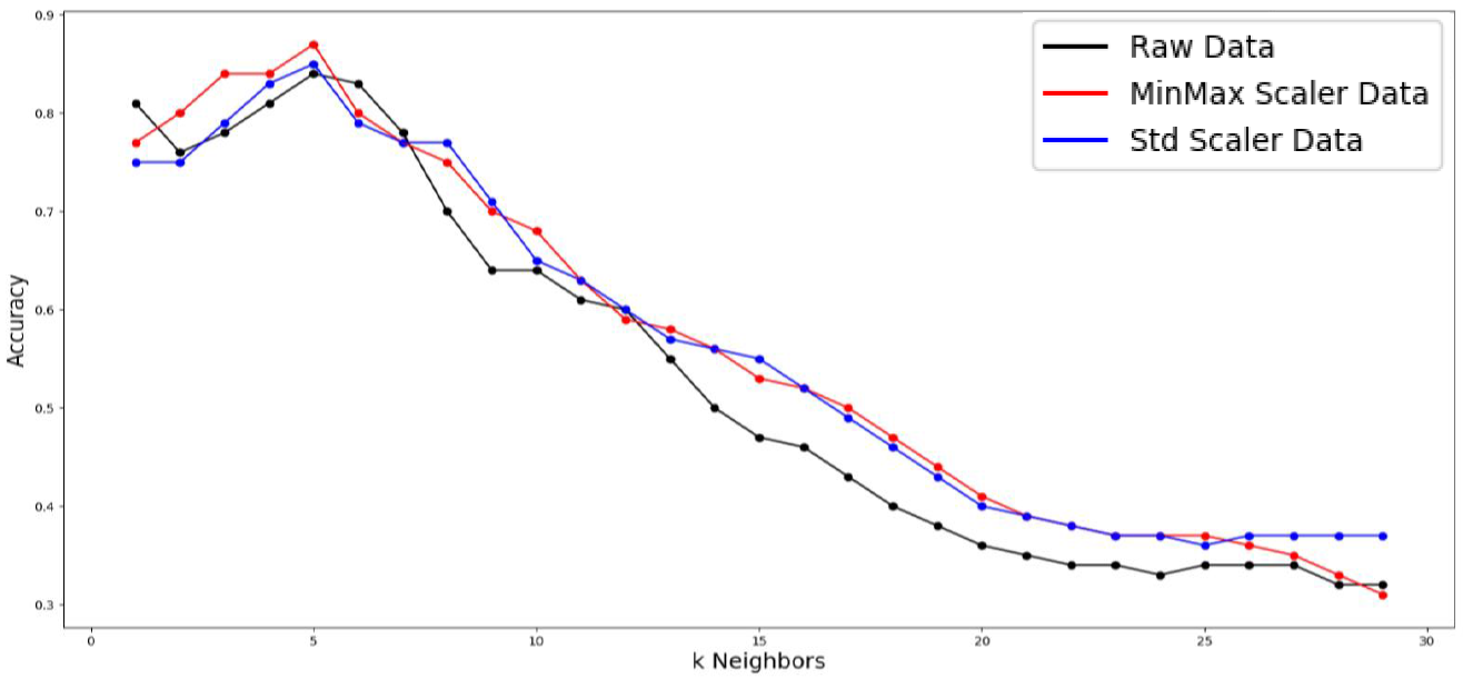
For each subject, 1 of their gait segments was randomly selected as holdout test data and the remaining were used as the larger training set resulting in a training sample size of 60 gait segments with class labels (subject IDs) and a test set of 10. The classification was run 1000 times for each k ranging from 1 to 29 to generate an average classification accuracy on the holdout test data. The score metric is the mean accuracy of all 10 test data samples with 1.0 being the best and 0.0 the worst. The entire training and testing runs were performed 3 times using different data scaling methods: raw features, min-max scaling 0 to 1, and standardization.
With a training sample size of 60 with 10 different class labels a maximum accuracy of 0.87 was achieved. The optimal k-neighbors value was 5 across all feature scaling methods. The table below shows the accuracy results omitting k values above 15 since accuracy only decreased as k grew larger as illustrated in the plot below.