This is the paper review of the following paper.
Lemme, Andre, René Felix Reinhart, and Jochen Jakob Steil. “Online learning and generalization of parts-based image representations by non-negative sparse autoencoders.” Neural Networks 33 (2012): 194-203.
This paper presents a variation of autoencoder (AE) models. It is estimated that the human visual cortex uses basis functions to transform an input image to sparse representation1.
Autoencoders seem to be good models for the process because they can produce embedding representation with different dimensions from the original signal. Training of the model is also easy because we don’t need labels for the inputs but use the difference from the original input and the recovered input from embedding as an error function.
There are many variations for the autoencoders, including variational autoencoder (VAE) and sparse AE. VAE is for the interpretability. Conceptually, the high-dimensional space of the embedding can have an arbitrarily complex pattern. There can be many undefined spaces. For example, let’s say there are four dimensions for embedding and it happens to represent a cat with [0.5 0.5 0.5 0.5 0.8] and a dog with [0.5 0.5 0.5 0.5 0.2]. But there can be no meaning between 0.2 and 0.8 for the last dimension. It becomes especially problematic when you want to generate some data by randomly sampling from embedding space. It will be embarrassing if there are no meaningful data to most of the embedding space. VAE solves this problem by adding the constraint that the embedding values should follow a gaussian normal distribution. Technically, you add additional loss term for KL divergence between the distribution of embedding values and gaussian distribution. You can see an online demo of generating an image from Doom by changing latent dimensions here.
Another meaningful variation is that making the embedding sparse. Here we want only a small portion of embeddings to be nonzero while standard AE and VAE generate dense representation. Why do we want sparse representation? Sparsity has many benefits.
- It is easier to interpret. You can think of each nonzero value as the feature present in the data. For interpretability, non-negativity helps, too. What will be the meaning of the negative yellow? Or negative car? My favorite representation is a sparse binary representation, which maximizes the interpretability.
- It is more biologically plausible. At any given point, about two percents of the neural cells are active. Of course, AI does not need to use the same mechanism as the rockets, helicopters, or jet airplanes do not use the flipping mechanism to fly as birds do.
- According to Olshausen and Field (2004), it can minimize the chance for destructive cross talk.
- According to Ranzato, Boureau, and LeCun (2008), it improves the linear separability.
L1 loss called lasso loss is commonly used to build a sparse model. Andrew Ng used the KL divergence between a binominal distribution and the activation frequency of embedding values. It has one additional parameter that allows us to set the activation probability. Therefore, we can set the activation probability of embedding at two percent that is about the same as how frequently the biological neural cells activate.
This paper presents a non-negative sparse autoencoder (NNSAE). Compared to other AE variants, NNSAE has the following benefits for my heterarchical prediction memory (HPM).
- Non-negative
- Sparse
- Online
- Sparsity adds a built-in regulation to prevent overfitting
- Local
Non-negative matrix factorization (NMF) has been used to get non-negative embedding. However, this method relies on iterative fitting and does not work well with streaming inputs. NNSAE uses a larger update rate for negative weights than positive weights. It penalizes the negative weights and forces the weights to be positive. The logistic activation function has been used to make the output values between zero and one. In NNSAE, the logistic activation function is shifted such that only a certain percentage of the cells are activated. The below figure explains this concept visually.
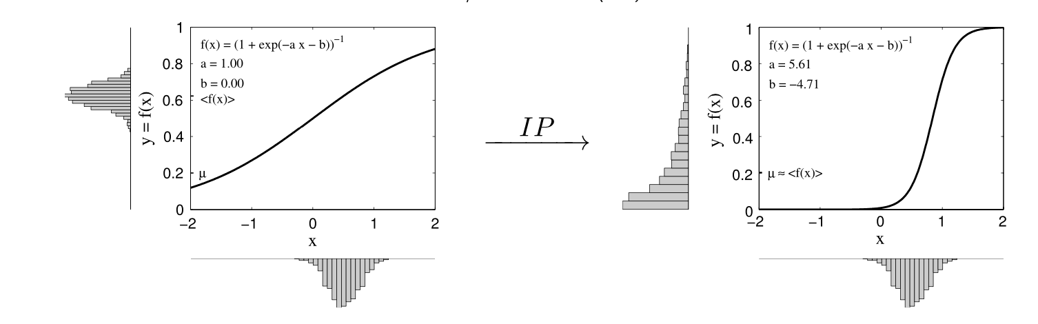
This figure explains how NNSAE generates a sparse code by shifting sigmoid function by parameter a and b. As can be seen in right figure, the shifted sigmoid generates a sparse code given gaussian input.
The sparsity constraint of the model enforces the regularization. In the synthetic toy dataset, where the ground-truth basis dimension is 18, we can see that the additional hidden dimensions are not used, as we can see when we use embedding dimensions larger than 18.
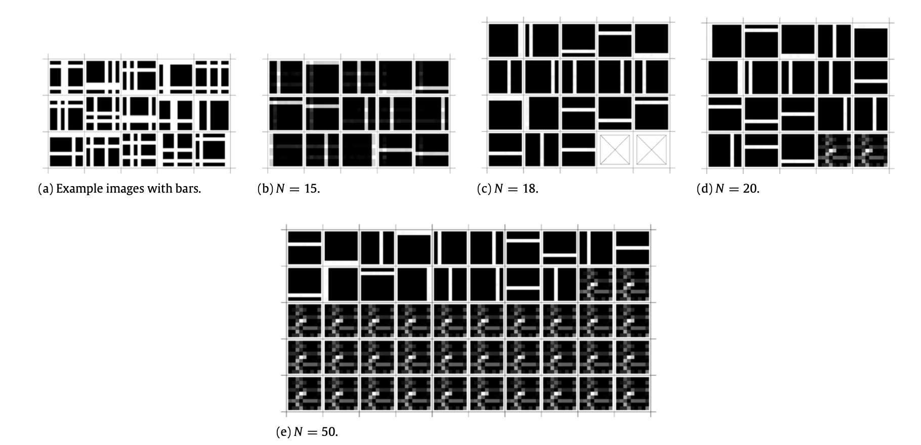
This sysnthetic dataset has 18 basis. As we can see in (d) and (e), when there are more hidden units, the model only uses 18 basis and does not use the remainder.
Similarly, for MNIST and CBCL face dataset, we can see that the number of used neurons does not explode beyond as the standard AE and sparsity is met.
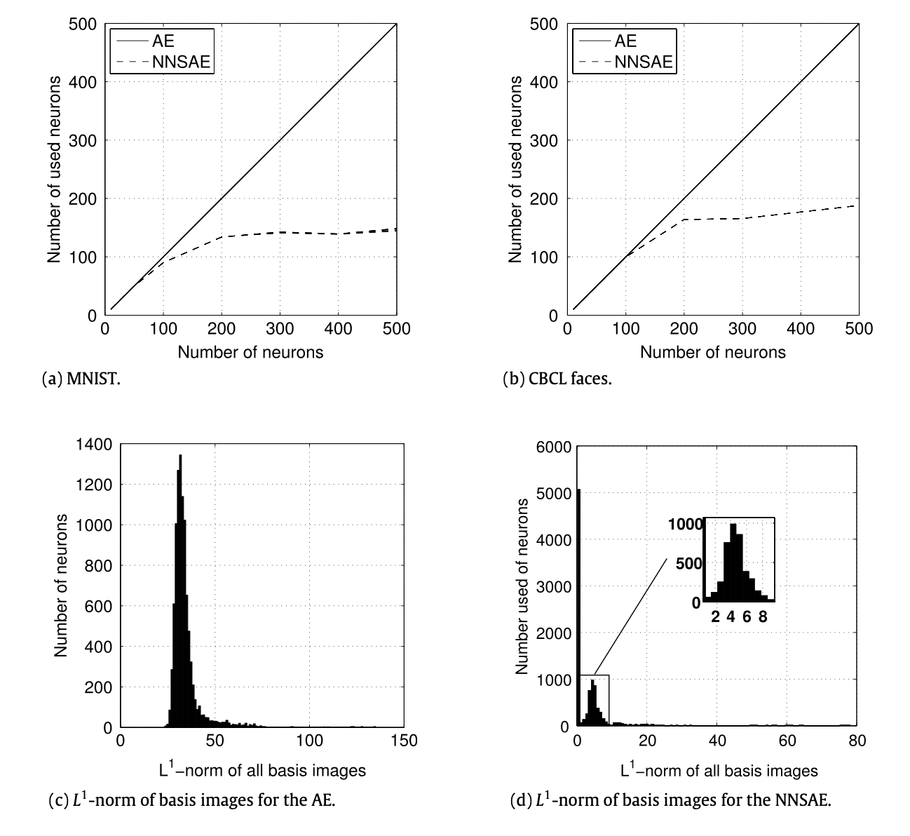
In (a) and (b), we can see that the number of used neurons for hidden unit saturates, even though the number of hidden units increase. In ©, we can see the standard AE uses all the basis, while the NNSAE uses only subset of basis and the remainder is near zero as seen in (d).
As the algorithm is online, we can change the dataset in the middle of the training and expect the model to adapt to the new dataset, as can be seen below.
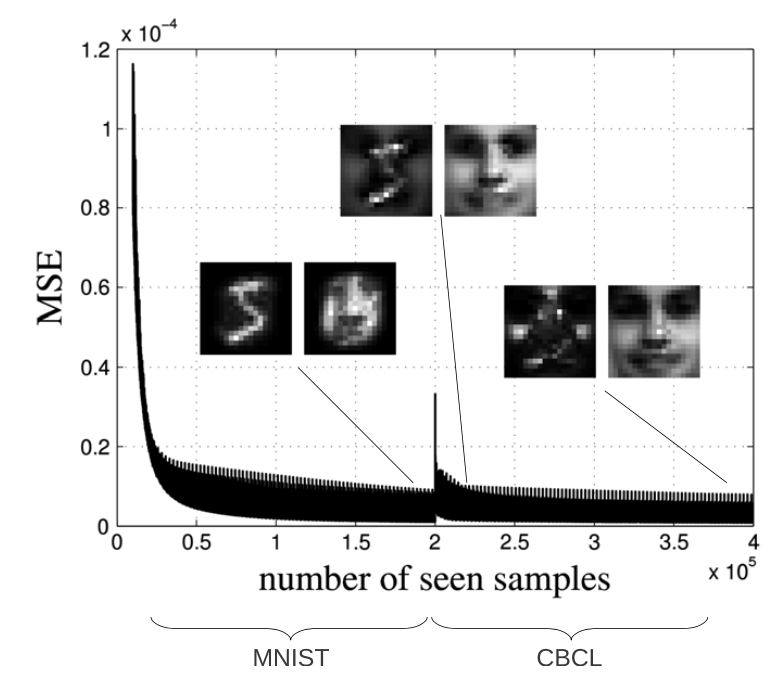
The algorithm is online, therefore when we switch the dataset, it adapts to new dataset.
Use of NNSAE for HPM
I conjecture that each module predicts what will come as an input for the next time step. It is similar to AE that we can train the model minimizing the difference between the current input and recovered output. However, it becomes difficult to predict far in the future. I want to overcome this limitation by having a hierarchy of layers predicting the next time step. Each layer predicts the next time step and aggregates the four-time steps. This aggregated input is then reduced to the dimension of single input using NNSAE. The upper layer feeds back this information to the lower layer. Therefore lower layers have two inputs. One is the actual input, and the other is context.
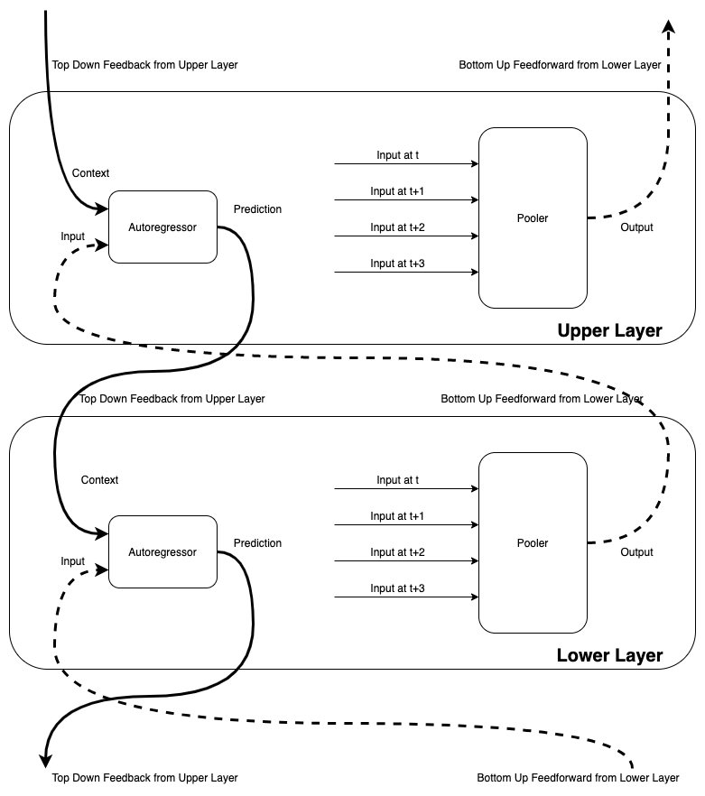
The diagram for HPM model
As a concrete example in the language modeling application, let’s say that you have a stream of characters. You might have three layers working on different time scales. The lowest layer L1 gets the characters encoded as sparse binary codes. In my experiment, I used 512 as the embedding size and only 10 bits, which is about two percents are on, and the rest is off. L1 tries to predict the next character by using a multilayer perceptron (MLP). But inherently, you cannot predict the next character given only the current character. For example, “a” or “h” can follow “c” as “cat” or “choice”. Context from the upper layer helps here. For L1, context from L2 contains information about the last four characters. Therefore L1 can predict the next characters better. Now, L1 sends a bottom-up feedforward signal by compressing embedding for four characters into 512 bits with ten on bits. This function is called “pooling,” and I used NNSAE for implementing the pooler.
The below figure shows my language model’s performance trained over a short text file and a large text file.
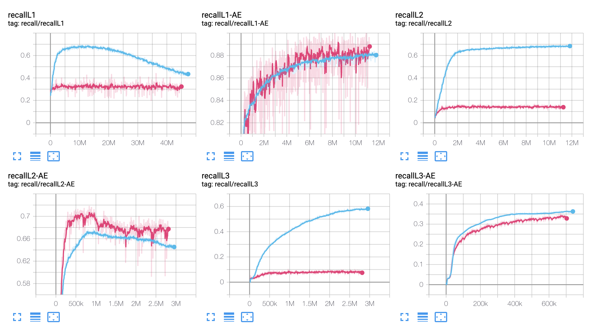
The performance of NNSAE for the character level language modeling. We used three layers. Each layer has a predictor and a pooler. Pooler uses NNSAE.
While the performance of the pooler or NNSAE is satisfactory, the predictor performance is not. Below are some of my future strategy to make the predictor faster and better.
- Deep Sparse Rectifier Neural Networks by Xavier Glorot, Antoine Bordes, Yoshua Bengio.
- Sparse deep belief net model for visual area V2 by Honglak Lee, Chaitanya, Ekanadham, Andrew Ng
- Synergies between Intrinsic and Synaptic Plasticity in Individual Model Neurons by Jochen Triesch
- Echo State Networks
- L1 Loss
Below is my mindmap for the related papers to artificial general intelligence.
- Olshausen, Bruno A., and David J. Field. “Sparse coding with an overcomplete basis set: A strategy employed by V1?.” Vision research 37.23 (1997): 3311-3325. ^